Why surrogate models fail when the geometry changes

TL;DR

This is the first blog in the series of explainers around Scientific Machine Learning.

We discuss the issues of training a vanilla deep neural network model on the simulation data. We then explain how these issues are solved and briefly introduce what surrogate models are.

In a conventional surrogate model, the node count of the training mesh is one dimension of a learned weight matrix. That count is a meshing decision. But it is not a property of the geometry.

That dependency has two effects:

1. The trained model operates at one resolution only.

2. The training pipeline must hold the node order constant across the dataset, which limits the geometry changes the model can learn.

Both effects are solved by using a larger model or a longer training run. This requires changing something fundamental.

1. The problem: why surrogate models are not in the design loop

A CAE simulation on an industrial case takes hours or days. A design study needs hundreds or thousands of iterations. Teams therefore truncate the study. They examine twelve variants when the design space contains thousands. Optimisation, uncertainty quantification and robustness studies are the first work that gets expensive because of cost of running.

A surrogate model promises to remove that constraint. It is trained one time on a set of completed runs. It is then evaluated in milliseconds. The idea is several decades old. Response surfaces, Kriging and POD-based reduced-order models all use it.

The problem, though, is that the promise is partly delivered. Where the geometry is fixed and only the parameters change, surrogate models operate in production today. Example: one duct shape, with the inlet velocity and the wall temperature as the variables. This work is routine.

Where the geometry itself changes, adoption is rare.

2. Change the geometry, and three complaints appear

Engineering teams report the same three symptoms:

• The model is accurate on the geometry family in its training data, and wrong outside that family.
• The model cannot use the completed runs that the company already has. Each surrogate project therefore starts with a new and expensive DOE campaign.
• The team cannot validate the model with the procedures that it already trusts. The grid convergence study is the main example.

These three symptoms have one root cause. The traditional machine learning algorithms where you take a bunch of cases and throw them at a neural network does not work. The number of mesh nodes and the order of those nodes are inside the weights of the model. The sections below show how each one arrives there.

3. Terminology

• N: the number of points or nodes in one case.
• Parameters: the learned matrices. The software loads them from disk each time that the model runs.
• Checkpoint: the file that contains the parameters. The checkpoint is the model.
• Discretisation: the operation that converts a continuous field into an array of values at selected positions.

4.How do nodes become weights?

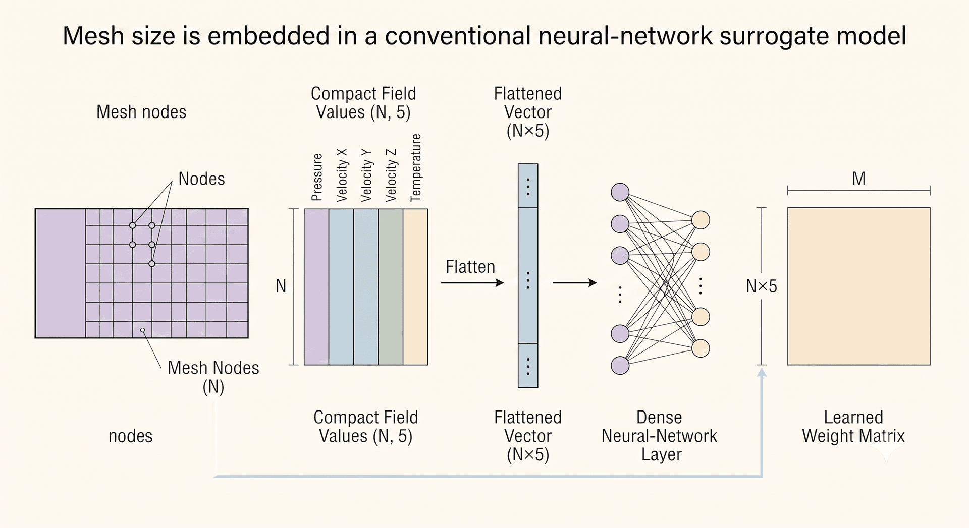
A completed run gives data for each node in the mesh. Each node has a position and five field values: Ux, Uy, Uz, p and T. A mesh with 400,000 nodes therefore gives an array with the shape (400000, 5).

A standard neural network cannot read that array. The basic component of a network reads a list of numbers with a fixed length, and writes a list with a fixed length. To use the array, you must first put all of its values into one long list. The array becomes one vector with 2 million values.

This component is a dense layer. It does one operation. It multiplies its input by a matrix of learned numbers, and sends the result to the next layer. The matrix contains the weights of the layer, and training adjusts these weights. The lengths of the two lists set the shape of the matrix. The shape becomes permanent when you define the model, and nothing can change it at run time. At the end of training, the software writes each matrix to the checkpoint.

Examine the size of that first matrix. If 400,000 nodes go into the input, the matrix has 2 million rows. If the model is built in the opposite direction, from design parameters to a field, the last matrix has 2 million columns. At an internal width of 512, which the model builder selected, this one matrix contains 1.024 billion learned numbers. In single precision it uses about 4 GB. It is much larger than all of the other matrices together.

In both directions, the number 400,000 became one dimension of a learned matrix. It goes into the checkpoint, and it stays there for the full life of the model.

5. Where the number 400,000 came from

The number 400,000 is the node count of one mesh. An engineer selects a base cell size, a growth rate, a number of prism layers, and a set of refinement regions. A second engineer, with the same CAD model and the same internal best-practice document, can select different values and be equally correct. Both meshes converge to the same duct. The airflow is identical in both cases.

The mesh is a property of the numerical method. It is not a property of the duct. A conventional surrogate model has written it into the weights.

Classical reduced-order models have the same defect. In a POD-based model, each mode is a vector with one value for each node. The number of nodes is in the modes, in the same way that it is in the weight matrix.

6. A geometry point should be the same for all cases

While the number of nodes is the direct problem, the order of the nodes is an indirect problem, and it puts more limits on the work.

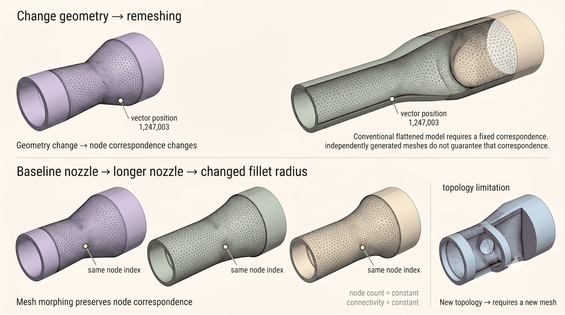
For example, 1,247,003 of the long vector meets row 1,247,003 of the weight matrix, and it meets no other row. During training, the numbers in that row learn a local rule. The rule can be equivalent to this statement: this position is immediately downstream of the outlet lip, where the pressure decreases quickly. The model learns the rule from the data only. The rule is correct only while value 1,247,003 refers to the same physical position in each case in the dataset.

For one fixed geometry the rule holds. A mesh generator gives the same order each time that it runs on the same CAD model. For different geometries the rule fails immediately, unless the data pipeline prevents the failure.

7. Mesh morphing: Deforming a baseline mesh per design

Teams prevent the failure with mesh morphing. One mesh is made for the baseline geometry. This mesh is then deformed to fit every other design in the study. The number of nodes and the connectivity do not change across the dataset. Only the positions of the nodes move. Value 1,247,003 would now refer to the same topological position in each case, and the model would train without a problem.

The cost of this method is in the data pipeline and not in the network. The model can see only the geometry changes that a morph operation can produce. A morph can make a nozzle longer. A morph can change a fillet radius. A morph cannot add a hole, remove a rib, change the number of grille slots, or accept a part from a different supplier. Those designs therefore produce no training case.

This is the true reason why conventional surrogate models fail to generalise across a design family. The capacity of the model, the optimiser and the training time are not the cause. The model learned the sample, and the team then rebuilt the pipeline to protect that assumption.

A larger network does not remove the constraint, because the constraint is in the shape of the first matrix. More training data does not remove it either, because the morph operation decides which cases can exist in the dataset at all. The defect is upstream of every hyperparameter.

8. The mesh is one sample of a field as a function

The velocity field in the duct is continuous. It has a value at each point in the fluid. This includes the points between the cell centres. It includes the point 0.3 mm downstream of the position where a node happened to fall. A mesh with 400,000 nodes contains 400,000 measurements of a quantity that has values at an infinite number of positions.

Consider the temperature in a room. One description is a list of 500 thermometer readings, each with a position and a value. A second description answers this question for any position in the room: what is the temperature here? It also answers it for the many positions where no thermometer was present. That second description is a function, and the 500 readings are one sample of it. Thermometers in different positions give a completely different list for the same room.

Engineers move between these two descriptions continuously, and they seldom stop to separate them. A solver calculates with the second description, because the governing equations are statements about a continuous field. The solver then stores the first description, because a computer must contain numbers in an array. The discretisation is the operation between the two descriptions.

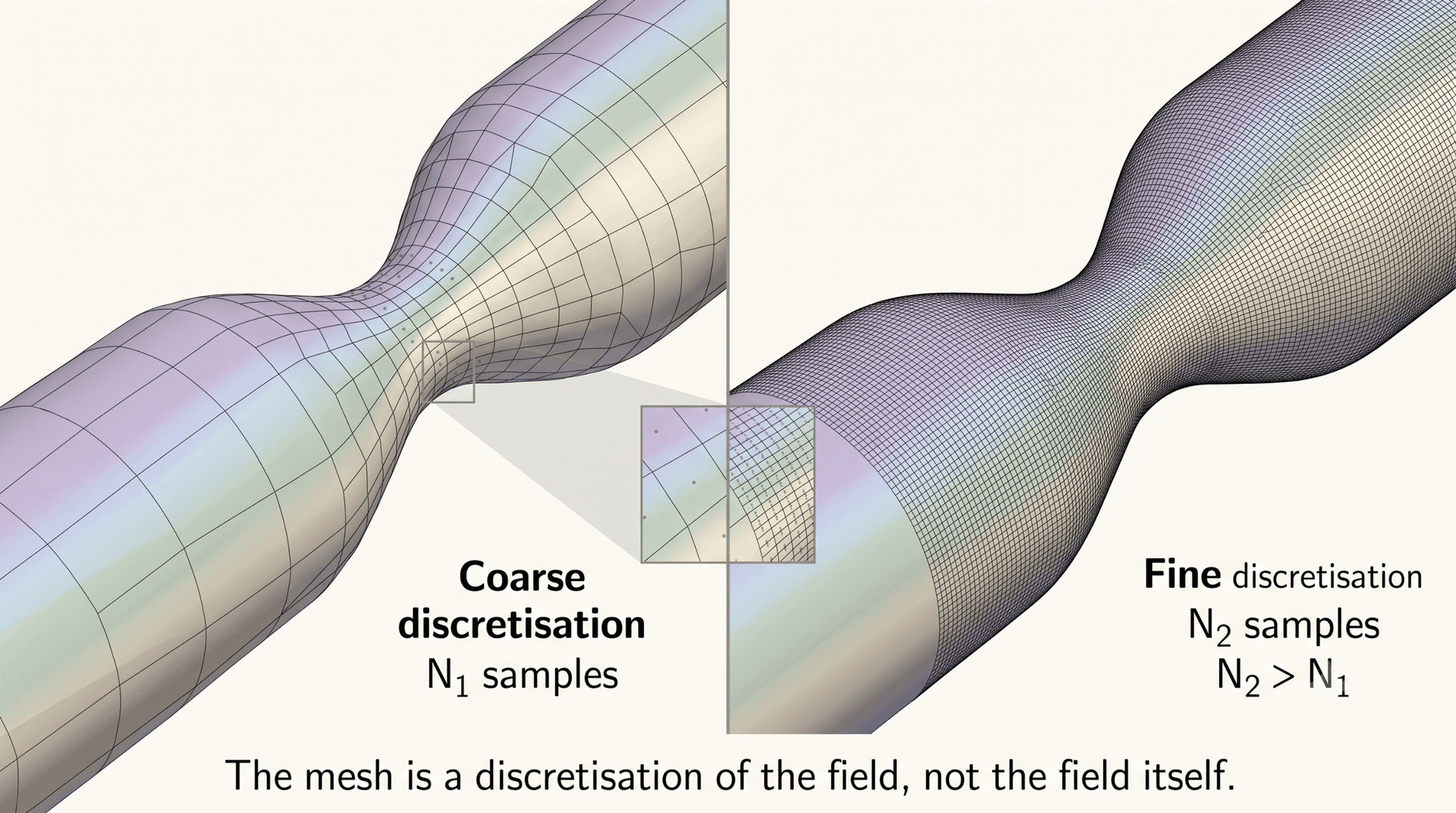
A conventional surrogate model learns from the first description and keeps it. The node count and the node order are properties of that one sample, and both are now parameters of the model.

9. How do we tackle these two problems using architecture change?

The node count sets a dimension of a learned matrix, so the trained model works at one resolution only. Flattening the field ties each row of that matrix to one position in the vector, so the dataset must keep the node order the same. Those are the two effects, and one question follows from them.

Can a model learn the mapping between physical fields without making the discretisation part of the learned parameters?

An architecture that does this exists, and the change is in where the weights are applied. One small matrix reads a single point: its position, and the direction that the surface faces there. The same matrix is then applied to the next point, and to the next, across the whole mesh. Its shape is set by the number of values that describe one point, and never by the number of points. A mesh with 400,000 points and a mesh with 4 million points use the same matrix.

Both effects mentioned above end there. No dimension has to match the input, so the resolution of a query becomes a choice made at run time. No row of weights belongs to one node, so the dataset has no reason to keep the node order the same. Mesh morphing stops deciding which geometries can enter the training set.

One step is still missing. A model built from that matrix alone would treat every point in isolation, and pressure could not be learned that way. A second step mixes information between the points, and its parameters are also independent of the point count.

The claim is then checkable. List the shape of every matrix that the model saved. If the node count appears in none of them, the model does not contain the mesh.

A model of this kind is a neural operator.

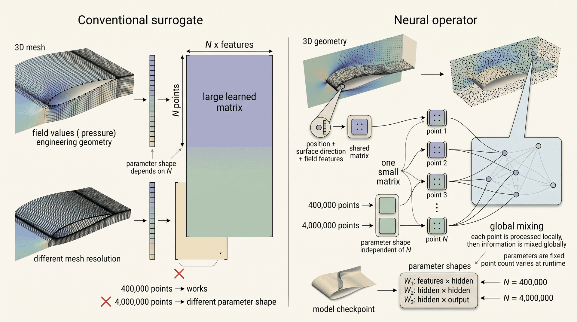
In the next blog we will discuss mechanism: the shape of each step, the operation that mixes the points, and what the properties help in achieving the resolution invariance and mesh independence.