Neural Operators for Engineering Simulation

TL;DR

This is the second blog in our "Scientific Machine Learning explainer" series. The first blog, Why surrogate models fail when the geometry changes, showed how a surrogate becomes tied to the mesh it was trained on. This post explains how a neural operator avoids that by addressing the following topics:

• A neural operator learns a mapping between fields. The number of points that represent a field is not part of the model.
• The learned weights do not depend on how many mesh points there are or on the order they are stored in.
• Two requirements follow. The model must treat every ordering of points the same way, and information must still travel between points across the domain.
• Larger meshes can use the same learned model, but they still create larger activations and higher runtime cost.

1. How does a Neural Operator work?

Take a battery-pack cooling problem. Each design case has its own geometry and its own mesh, but every case is the same physical problem: predict how heat moves through the domain.

The model sees the domain as a set of sampled points. Each point carries a set of features which are the model inputs:

• Coordinates (`x, y, z`), which locate the point in the domain.
• Surface normals (`nx, ny, nz`), which give the local orientation of a surface.
• Material properties, which identify the region the point belongs to (fluid, cell, casing, cold plate) and can include values such as thermal conductivity or density.
• Boundary-condition features, which describe the physics imposed at that location: inlet velocity, inlet temperature, wall temperature, heat flux, or a no-slip condition.
• Operating conditions, which hold case-level settings such as coolant flow rate or heat generation.

For training, these inputs form a tensor of shape (B, N, F):

• B simulation cases in a batch
• N sampled points per case
• F features per point

The model’s output is a prediction of the physical fields over the same points, such as temperature T, velocity components U, V, W, and pressure P.

The learning problem can be defined as:

geometry + material + boundary and operating conditions → Fields

This is the useful starting point for understanding a neural operator: it is not learning a fixed vector-to-vector relationship. It is learning a mapping between physical fields represented at spatial locations.

To be able to use a model for generic mesh data, neural operators came into existence. But they introduce two issues that must be solved for a successful implementation:

• Permutation equivariance
• Interaction between spatial points

Both of the issues mentioned above are discussed in detail below. But let us start with how mesh independence is achieved first.

2. Mesh independence through lifting operations

For the learned weights to stay independent of N, which is the number of sampled points per case (mesh points / number of cells), the model must never see the whole mesh as one vector. It works on one point at a time.

The first step is a lifting operation. It takes the F features at a point and maps them into a wider latent representation, for example from 6 input features to 128 latent features. The same learned transformation is applied at every point. Its size depends on the number of features and on the latent width, and on nothing else.

The mesh decides how many point representations exist. The weights decide how each one is encoded. A case with 200,000 points and a case with 600,000 points pass through exactly the same lifting layer.

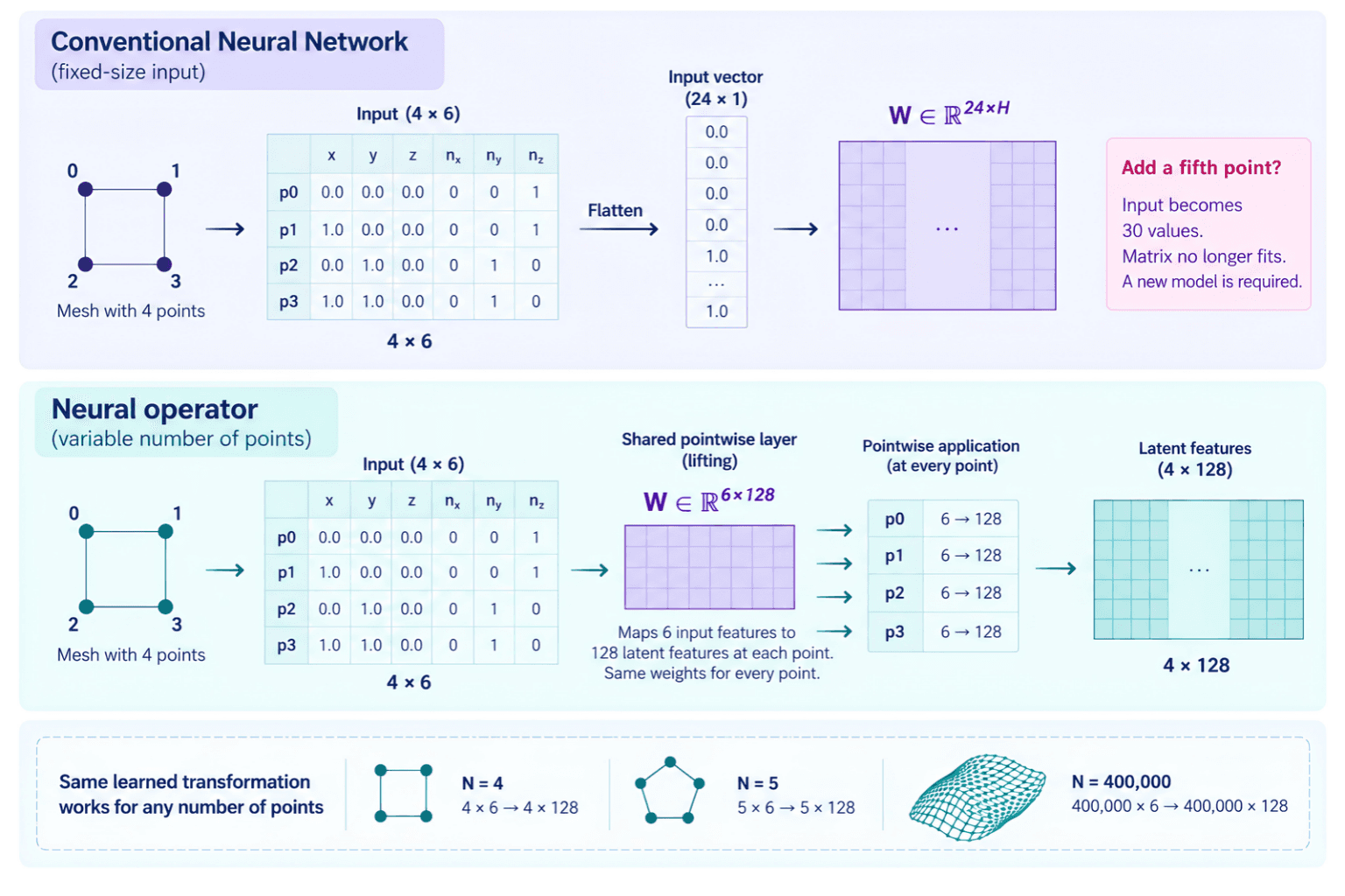
This removes the fixed point-count constraint. The next requirement is that the model must also remain valid when the ordering of those points changes.

3. Permutation equivariance: order carries no physics

A mesh file has a storage order, but that order has no physical meaning.

Point 17,432 is not important because it appears in row 17,432. Its physical identity comes from its coordinates, geometry, material properties, boundary conditions and other features.

The model should therefore behave consistently even if the input rows are reordered.

The model must give the same answer whatever order the rows arrive in. If the input points are shuffled, the output fields must shuffle in exactly the same way, and the predicted field itself must not change. This property is called permutation equivariance.

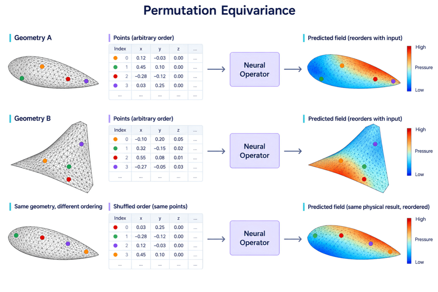
For engineering datasets, this removes another fixed-mesh constraint. Different simulation cases do not need a shared node numbering simply for the network to process them.

Point 17,432 in one geometry does not need to correspond to point 17,432 in another.

At this stage, the model can handle both a variable number of points and a variable ordering of those points.

But each point has still only been encoded locally. A physical field cannot be predicted from isolated point representations alone.

4. Interaction between spatial points: information must travel across the whole domain

The next requirement is interaction between points which are separated in the domain by a large distance but still can affect the field data to be predicted at that point.

After the lifting step, every point has its own latent representation. That representation contains local information, but the physics is coupled across space.

In incompressible flow, for example, a restriction in one part of the geometry can affect the pressure field much farther away. Downstream behavior depends on what happened upstream.

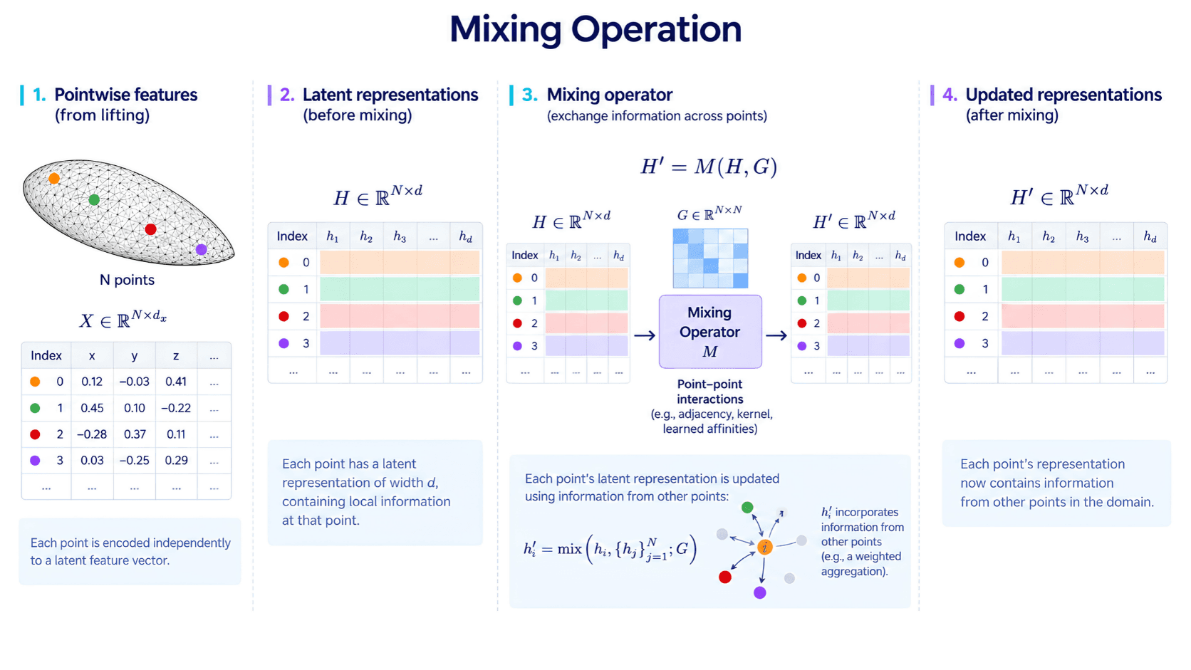
The model therefore needs a mixing operation that allows the representation at one location to depend on information from other locations.

In general, this can be written as:

H' = M(H, G)

where

• H contains the latent representations at all points,
• G describes the spatial or geometric relationships used by the model,
• H' contains the updated representations after information has been exchanged.

Lifting, permutation equivariance and mixing together give a model that works on any compatible mesh. What remains is the cost of doing so.

5. Compute scales with the mesh, even when the model does not

Once the point representations are created and mixed, the main scaling question is straightforward: how much intermediate data does the model have to process?

A larger mesh creates larger activations. If the latent width is 128:

• 200,000 points → 200,000 × 128 latent features
• 600,000 points → 600,000 × 128 latent features

The second case therefore requires more memory and more work in every operation that acts on those representations.

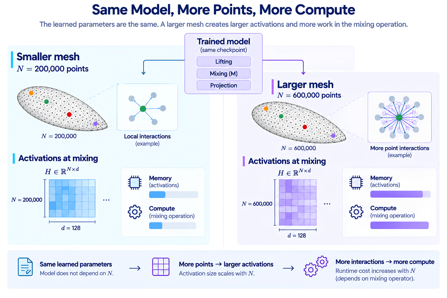
The exact cost depends on the mixing strategy:

Local or sparse mixing can scale relatively close to the number of points, while dense pairwise mixing grows much faster because the number of possible interactions increases with N².

So the architecture has to balance two things: keeping the model flexible enough to work across changing discretizations, while keeping the cost of processing those points manageable.

That trade-off matters because the value of a neural operator is not only architectural. It changes how simulation data can be reused, how quickly designs can be iterated and how much preprocessing is needed to make different cases fit the same ML workflow.

6. Advantages of the Neural Operator in a Workflow

The two properties change how simulation data is created and reused.

• Historical simulation archives are rarely uniform. Meshes change as geometries, meshing practices and refinement strategies evolve. A single model operates on any mesh type and size / count without a change to its learned parameters/architecture.
• At inference, the evaluation resolution is no longer dictated by the training resolution. A field can be sampled on a finer or coarser set of points than the model was trained on.

There are limits to this argument, though. A finer inference mesh cannot recover physics that was missing from the training simulations, and a larger mesh still costs more to evaluate, as section 5 showed.

7. Where we go next

• Neural operators learn physics by learning the functions, hence the name operators. They still need an efficient way to move information across the domain.
• Different architectures solve that differently.
• In the next post we look at FNO, Transolver, GeoTransolver, AB-UPT, DoMINO and graph-based approaches, and follow how information moves through each one.