Putting Surrogate Models to the Test: GeoTransolver and AB-UPT on PLAID

TL;DR

• Our last post explained how surrogate architectures work. This one puts two of them, GeoTransolver and AB-UPT, to work in Curlscape Sift, the platform we built to train surrogate models.
• We tested them on PLAID, a public set of engineering simulation datasets on which six other methods have already been scored. That lets us compare our models with other people's work on the same data.
• GeoTransolver beat AB-UPT on all five datasets.
• Against the six published methods, GeoTransolver usually landed in the middle of the table. Its best finish was 3rd out of 8, and its worst was 6th.

The Results at a Glance

We begin with the outcome and explain how we arrived at it in the sections that follow. The table below compares the average field error of eight methods on five PLAID datasets. Six of these methods are the reference results published with PLAID. The remaining two, GeoTransolver and AB-UPT, were trained and evaluated in Curlscape Sift using a single shared training recipe.

The error is PLAID's relative root mean square error, averaged over the same output fields for every method. Lower values indicate better predictions, with the lowest error in each row highlighted in bold. The final column gives GeoTransolver's position among the methods evaluated for that dataset.

The clearest pattern is that no single method leads across every dataset. MARIO records the lowest error on three datasets, while MMGP and Augur lead on one each. Of our two models, GeoTransolver achieved lower errors than AB-UPT on all five datasets and placed between third and sixth among the eight methods. The porous-material dataset, where the topology changes from one sample to the next, proved the most difficult for both.

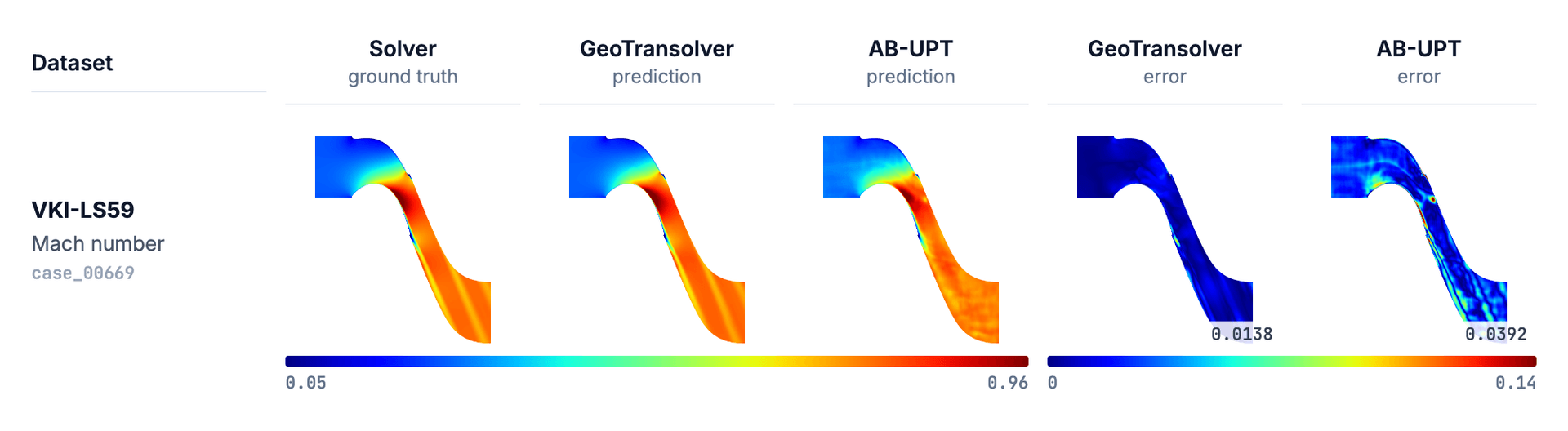
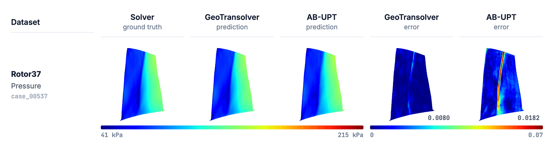
These are not official leaderboard scores. Because PLAID keeps its test targets private, our models were trained on less data and evaluated on cases we held out ourselves. Section 4 explains these differences in detail, and Section 5 examines what the results reveal about each dataset. Before that, the sections below explain why comparisons like this are difficult to make, and how Sift helps.

1. From Understanding Architectures to Evaluating Their Performance

Architecture papers often conclude with benchmark tables showing their proposed model outperforming alternatives. These results are valuable, particularly when the datasets, training choices and evaluation metrics are clearly documented. However, comparing conclusions across papers is rarely straightforward. One model may lead on a particular dataset, while another performs better under different conditions or is evaluated using a different metric. For an engineer trying to select a surrogate for their own simulations, the practical question remains: which architecture is likely to work best for the problem at hand?

In our third post, we examined nine surrogate architectures from the inside, looking at how they represent inputs, exchange information across a domain and generate predictions for new designs. That architectural perspective helps explain what makes each approach different, but it does not establish how well the models perform on a shared engineering task. We therefore move from theory to evaluation in this article, using Curlscape Sift to test GeoTransolver and AB-UPT on the public PLAID benchmarks. A subsequent article will extend this evaluation to our own engineering datasets.

2. How Sift Makes Architecture Comparisons More Reliable

Comparing two surrogate models should be as simple as training them on the same data and measuring their predictions. In practice, however, each architecture often comes with its own repository, preprocessing steps and training pipeline. Even small differences in mesh sampling, field normalization or dataset splits can affect the outcome, making it difficult to separate model performance from differences in the workflow.

We built Curlscape Sift to provide a consistent way to prepare simulation data, train different architectures and compare their results.

One dataset, multiple architectures

Sift stores each imported simulation case in a common format, including point coordinates, distance to the nearest wall, physical fields and case-level parameters. Cases can still have different meshes and point counts, as discussed in our first and second posts. Once registered, the dataset stays unchanged.

DoMINO, Transolver, GeoTransolver, AB-UPT and MeshGraphNet can therefore use the same case files and training, validation and test splits. The architecture and optional physics loss are run settings, rather than reasons to build separate pipelines.

Results we can revisit and compare

Every run preserves its configuration, case split, loss history and evaluation results. Sift evaluates the predicted fields across all points of held-out cases, while its design explorer lets users vary design parameters and inspect how the predicted flow changes. A trained model can also be tested against a separate dataset to assess how well it generalizes.

Testing the workflow with PLAID

PLAID was developed independently of Sift, making it a useful test of this process. We imported five PLAID datasets and completed ten training runs.

Each result remains linked to the data and settings that produced it. Even an early GeoTransolver run that failed to converge was retained, allowing us to investigate what went wrong rather than losing the experiment when we retrained. With that workflow in place, the next step was to understand what PLAID actually tests.

3. Why PLAID Provides a Useful Test of Generalization

PLAID (Physics-Learning AI Data model) was released in 2025 by a team at Safran, the aircraft engine and equipment maker. It is three things at once: a common format for simulation data with an open-source library, a set of datasets on Hugging Face, and a standing public leaderboard to which anyone can submit predictions.

PLAID is useful here for four reasons:

• Engineering relevance. Its problems include compressor and turbine blades, transonic flow, tensile loading and deformation of porous solids, generated using established simulation solvers such as elsA.
• Changing geometry. Shapes vary from case to case, and the porous-material dataset even changes topology as the number of pores changes. This directly tests the difficulty introduced in our first post.
• Consistent evaluation. PLAID defines training and test splits and an error metric, keeps official test targets private, and offers nested training subsets for studying the effect of data volume. Its open leaderboard provides an ongoing reference; the paper reports over 80 community submissions at the time of writing.
• Published baselines. The paper reports field-level results from six methods, giving us an external reference instead of comparing only against our previous runs.

Those six methods cover quite different approaches: MeshGraphNet (MGN), a graph network; MMGP, which morphs samples onto a common mesh before fitting a Gaussian process; Vi-Transformer and Augur, which work with mesh patches; FNO, a Fourier Neural Operator; and MARIO, a neural-field method conditioned on a compact code learned from each shape's signed distance field. That compact shape representation becomes especially relevant when topology changes.

For this study, we evaluated five of the six scored datasets. We have not yet run the sixth, 2D_ElastoPlastoDynamics, which involves transient behavior.

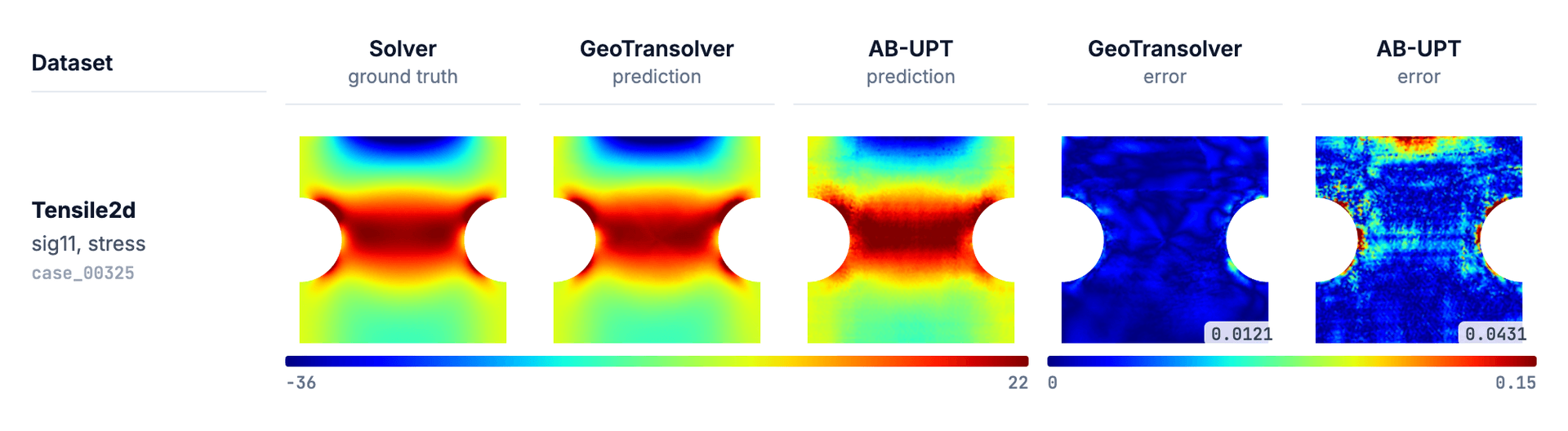
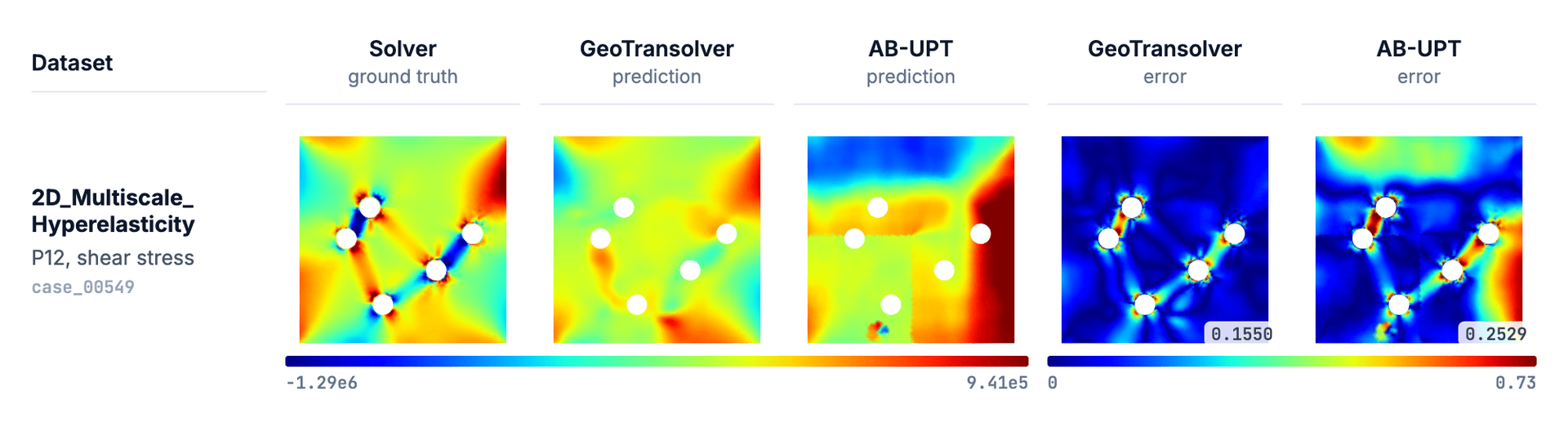
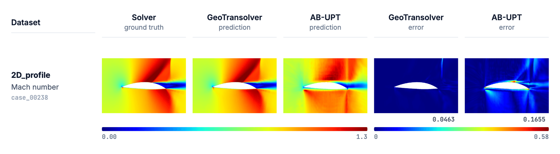
These datasets test different kinds of generalization. Rotor37 is a 3D compressor benchmark with density, pressure and temperature at 29,773 blade-surface points. 2D_profile isolates the effect of shape on near-sonic flow, including possible shocks, while VKI-LS59 adds turbulent viscosity prediction. Tensile2d and 2D_Multiscale_Hyperelasticity shift the focus to stresses and displacements in solids. Together, they let us compare architectures across more than one type of physics.

4. Our Evaluation Setup and How It Differs from the Published Benchmarks

Before interpreting the results, it is important to explain where our evaluation differs from the published PLAID experiments. These differences affect the degree to which the numbers can be compared directly.

Different training and evaluation samples

The first difference concerns the evaluation split. Because the official test targets are private, we could not calculate official leaderboard scores locally. Instead, we reserved a portion of the publicly available training data for evaluation and excluded those cases from model training. Where PLAID provides nested subsets, such as train_250 within train_500, we trained on the smaller subset and evaluated on the additional samples in the larger one. For the remaining two datasets, we held out a fixed random 20%. Consequently, our models trained on approximately 50% to 80% of the data available to the published methods, and our evaluation cases were not the same as the official test cases.

Our training counts above also include the samples used for validation, which is another important qualification when comparing them.

Comparing the same predicted fields

The second difference concerns the quantities being scored. PLAID uses a relative root mean square error, normalizing node-level prediction errors by the maximum value of the corresponding true field in each sample. This allows quantities such as pressure and displacement to be compared on a common scale. However, PLAID's overall score also includes global quantities, such as compressor efficiency, that our models do not predict. Because these quantities can be easier to estimate than spatial fields, including them could make the comparison misleading. On Rotor37, for example, every published method has a better overall score than its field-only score. We therefore compare our average field errors with the averages calculated from the same fields in PLAID's published per-field results, evaluating every mesh node.

We also independently checked the scoring process. Predictions are saved to files, after which a separate calculation recomputes the error from those outputs. This verification caught two concurrent scoring jobs on Rotor37 that produced a 0.2% disagreement between the reported and recomputed errors. Although the discrepancy did not affect the conclusions, we repeated the evaluation in isolation and obtained matching results.

The normalization also creates a special case for the field q in Tensile2d. Because q is exactly zero for most samples, dividing by a peak value close to zero can amplify small absolute errors into extremely large relative errors. Our models returned errors of 137 and 446 on this field, while the errors for other fields were only a few hundredths. PLAID excludes q from its published per-field table, and we follow the same convention.

One training recipe across datasets

The third difference is that we did not tune configurations separately for each dataset. Both architectures used 256 hidden channels, eight layers, eight attention heads, the same optimizer and the same small physics loss throughout the study. Their learning rates differed, following an issue observed in the first GeoTransolver experiment on Rotor37. When we initially used AB-UPT's learning rate, GeoTransolver collapsed to predicting approximately the same mean value at every point for seven epochs. Reducing the learning rate and introducing a short warm-up resolved the issue, and we retained those settings across all five datasets. This was a shared configuration comparison rather than a dataset-specific hyperparameter search.

5. What the Results Reveal Across Five Engineering Problems

The results table at the top of this article compares the average field error for each method across the five datasets. With the evaluation setup explained, the patterns behind those numbers can now be examined more closely.

The most important observation is that no single method leads across every dataset. MARIO records the lowest error on three datasets, while MMGP and Augur lead on one each. However, MARIO's strong results on the flow problems do not carry over to the porous material dataset, where it ranks last among the published methods. This variation reinforces a central point of the series: performance depends on the geometry, physics and data characteristics of the problem, so a ranking obtained on one benchmark should not be treated as a universal recommendation.

GeoTransolver performed best relative to the other methods on VKI-LS59, finishing third of eight behind MARIO and Vi-Transformer, but ahead of FNO, MMGP, MeshGraphNet and Augur. Turbulent viscosity contributed much of the error for our models and nearly all published methods, with Augur being the exception. On 2D_profile, where geometry is the only input, GeoTransolver's error of 0.0429 was very close to Augur's 0.0425; given the evaluation differences, that gap is too small to support a meaningful ranking between them. AB-UPT struggled more on this dataset, with validation loss stabilizing near 0.48 from approximately epoch 200, while GeoTransolver continued improving toward 0.05. On Rotor37, GeoTransolver ranked fifth and recorded roughly 1.3 times the error of Vi-Transformer, despite having trained on only half as many cases as the published methods.

Tensile2d tells a different story. MMGP and MARIO substantially outperform the remaining methods, with errors approximately four to seven times lower than those of the other approaches. In this dataset, every sample can be morphed onto a common reference mesh, making MMGP's geometric alignment strategy particularly effective. GeoTransolver ranked sixth, although its error was still about three times lower than MeshGraphNet's despite using half the published training data. The result illustrates why mesh morphing remains an important baseline when the geometry family permits it.

Why changing topology remains difficult

The most challenging dataset for our models was 2D_Multiscale_Hyperelasticity, where the number and arrangement of pores vary between samples. Because the topology changes, MMGP cannot establish the common reference mesh it requires and therefore cannot be applied. MARIO also performs poorly relative to the other published methods, suggesting that compressing such varied geometries into a short shape code may be difficult in this setting. Our models encountered similar challenges: GeoTransolver's error was approximately five times that of Augur, and neither GeoTransolver nor AB-UPT reached a low validation loss. Although Augur achieved the best result here, the dataset highlights how topology changes can expose limitations in otherwise effective surrogate approaches.

What averages can hide

Average errors also conceal variation between individual test cases. On Rotor37, AB-UPT produced more consistent errors across blades, with its worst case only 1.65 times its median error. GeoTransolver achieved lower errors on typical blades, but its worst case was 2.9 times its median. Interestingly, both models struggled on the same blade, suggesting that this particular case may be unusually difficult rather than pointing to a failure unique to one architecture. Examining this distribution therefore adds context that a dataset-level average cannot provide.

Another useful pattern emerges when errors are examined field by field. Our models struggled with many of the same quantities as the published approaches: a stress component in Tensile2d, shear stresses in the porous material, turbulent viscosity around the turbine blades, and density and pressure on the compressor. This agreement does not establish that the models have learned the underlying physics correctly. Nonetheless, it suggests that their difficulties are not entirely arbitrary and may reflect challenges inherent to the physical prediction tasks.

6. GeoTransolver vs. AB-UPT: Accuracy, Training Cost and Architectural Fit

Accuracy versus training cost

Within our shared experimental setup, GeoTransolver consistently achieved lower errors than AB-UPT across all five datasets and every predicted field, with an advantage ranging from approximately 1.8 to 3.5 times. AB-UPT, meanwhile, placed seventh or eighth on each dataset. However, the accuracy advantage came with a computational cost: on Rotor37, a GeoTransolver training epoch took 76 seconds compared with 31 seconds for AB-UPT. Model selection therefore involves a trade-off between prediction accuracy and training expense, even before considering deployment requirements.

The Rotor37 training curves help explain this difference. AB-UPT's training and validation losses converged to similar values and remained nearly flat for the final thirty epochs, suggesting that additional epochs alone were unlikely to improve performance under the chosen configuration. GeoTransolver behaved differently: its training loss continued decreasing after its validation loss had stopped improving, indicating overfitting. Even so, its evaluation error was roughly half that of AB-UPT. This leaves open the possibility that additional training data could help GeoTransolver generalize better, although that would need to be tested directly.

Why this is not a universal verdict on AB-UPT

These results should not, however, be interpreted as a general verdict against AB-UPT. The architecture was developed for 3D automotive aerodynamics involving millions of points per case (Alkin et al., 2025), whereas PLAID meshes contain roughly 4,000 to 39,000 nodes and four of the five datasets are 2D. We also fixed the anchor count at 2,048 without testing alternatives. For Rotor37, this meant representing 29,773 surface points through 2,048 anchors, and a different anchor configuration could potentially change the outcome. Our conclusion is therefore specific to this experiment: under a shared, largely untuned training recipe, GeoTransolver (Adams et al., 2025) delivered better accuracy on these PLAID problems, but required approximately twice the training time.

7. What We Can Conclude, and Where the Comparison Has Limits

How to interpret these results

The results presented here are not official PLAID leaderboard scores. Our models were trained on smaller datasets, evaluated on internally held-out samples, compared using field-level metrics and trained only once per configuration. Small numerical differences, such as the gap between GeoTransolver and Augur on 2D_profile, should therefore be treated as effectively inconclusive. This is especially important for 2D_profile, where the evaluation contains only 60 samples and the estimates are consequently more sensitive to the sample selection. In addition, our runs included a small physics loss that the published methods did not use; we have not yet performed an ablation to determine whether it improved performance in this study.

Within those limitations, the results still provide useful context. GeoTransolver's error is within a factor of 2.5 of the best published transformer on four of the five datasets, and it outperforms MeshGraphNet on four. At the same time, it does not achieve the lowest error on any dataset. Establishing an official benchmark position would require training on the complete published training sets and submitting predictions to the PLAID leaderboard. Until then, the comparisons are best understood as an informative internal evaluation against published reference results.

What engineers can take away

For engineers selecting a surrogate architecture, several practical lessons emerge. When all designs can be mapped reliably onto a common mesh, a morphing-based approach such as MMGP deserves consideration as a baseline. Where topology changes, the results suggest anticipating a more difficult learning problem and assessing whether additional training data are needed. For flow predictions around changing geometries, GeoTransolver appears to be a reasonable candidate for initial experiments. Nevertheless, none of these observations replaces validation on the intended application. The most relevant model is ultimately the one that performs reliably on the geometries, operating conditions and physical fields that matter to the engineering team, and Sift is designed to make those comparisons repeatable.

Testing Surrogates on Industrial Engineering Datasets

Public benchmarks provide valuable external reference points, but engineering teams ultimately need to understand how surrogate models behave on the simulations they work with every day. In the next article, we apply the same evaluation approach to two engineering datasets in Curlscape Sift. The first involves an air-cooled PCB with a heatsink, where we compare GeoTransolver, AB-UPT and DoMINO both with and without the physics loss. The second focuses on battery cold plates spanning seven channel families. By excluding an entire channel family from training, we can investigate how each model responds to a design family it has never encountered. Together, these experiments will take the discussion beyond public benchmarks and toward the generalization questions that matter in practical engineering workflows.

Earlier posts in this series

Why surrogate models fail when the geometry changes

Neural Operators for Engineering Simulation

A Comprehensive Review of Different Surrogate Architectures