
Many cheap runs, a few expensive ones, one corrected model
Co-Kriging learns how a fast, biased simulation differs from a slow, accurate one, then applies that correction across the design space. Two studies below, with the errors measured on runs the model never saw.
01Method
How the fusion works
It works when the cheap model is wrong in a consistent way. In both studies below, the cheap and expensive results were strongly correlated.
- 01
Run many cheap cases
A coarse mesh or a lower-order method (BEMT, 1D) sampled across the whole design space. It is biased, but the bias is smooth.
- 02
Run a few expensive ones
A small nested set of fine-mesh or full CFD runs at points that were also run cheaply, so each pair shows the discrepancy directly.
- 03
Learn the correction
Co-Kriging models the expensive response as a scaled cheap response plus a Gaussian-process correction, f_HF(x) = ρ·f_LF(x) + δ(x).
- 04
Check it out of sample
Hold fine runs out, refit, predict them, and report the error against the raw cheap model. The trained envelope is part of the result.
02Study 1 · Electronics thermal
1U server board, coarse vs fine mesh
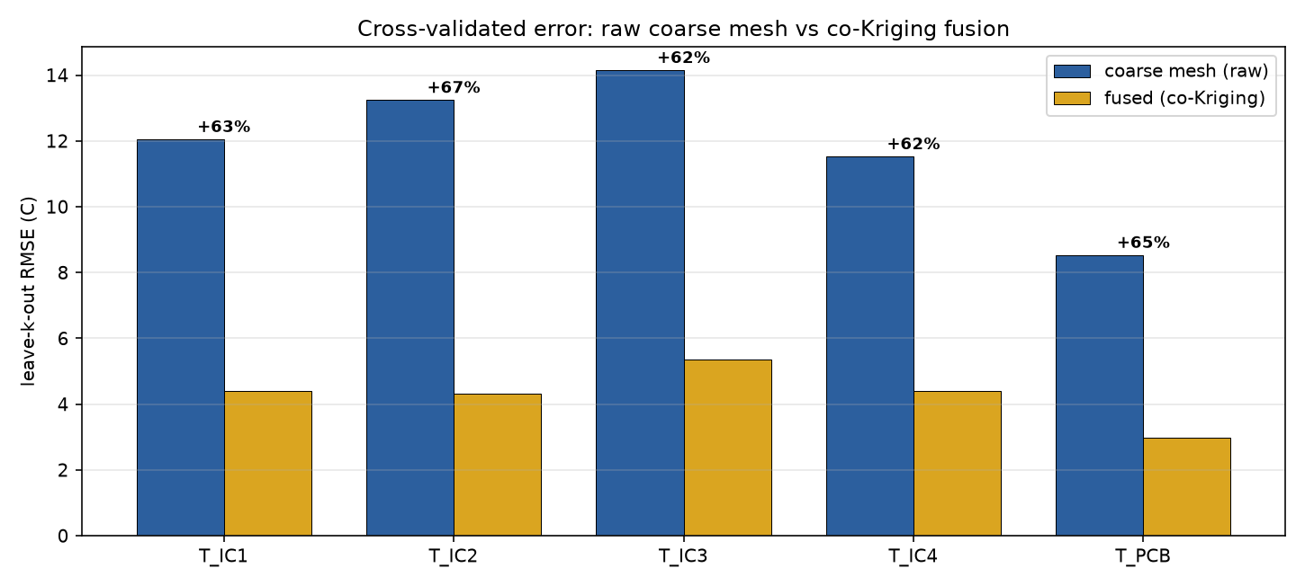
200 coarse-mesh and 10 fine-mesh conjugate-heat-transfer runs, fused per component. Leave-2-out cross-validated RMSE fell by 62–67% against the raw coarse mesh, for example from 12.05 to 4.40 °C on CPU 1.
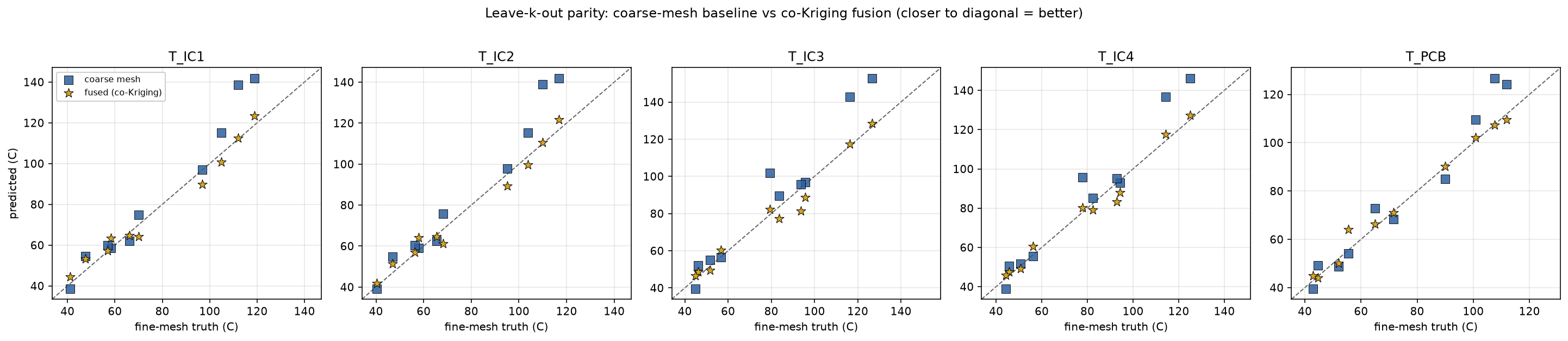
The coarse mesh tracks the fine one closely (Pearson r 0.97–0.98, Spearman 1.00 on the pilot points) but runs hot at high power and low airflow, where it under-resolves the boundary layer. That is a smooth bias, which is what co-Kriging corrects.
Setup
- Solver
- OpenFOAM v2506, chtMultiRegionSimpleFoam (steady conjugate heat transfer)
- Geometry
- 1U server board: PCB, 4 ICs, air
- Low fidelity
- 200 runs, 4 mm mesh, ~119k cells
- High fidelity
- 10 runs, 1.5 mm mesh, ~2.3M cells, each also run on the coarse mesh
- Inputs
- CPU power 20–80 W · chip power 15–60 W · inlet velocity 1–5 m/s · inlet air 15–45 °C
- Outputs
- Volume-averaged temperature of each IC and the PCB
- Sampling
- 200-point Latin hypercube (thinned to 120 for the fit); 10-point maximin LHS, nested
- Model
- SMT MFK co-Kriging, one per output, Matérn-3/2, unit-cube normalisation, nugget 1e-6
- Validation
- Leave-2-out cross-validation on the 10 fine-mesh points
Results, leave-2-out on 10 fine-mesh points
| Output (volume-avg.) | RMSE coarse °C | RMSE fused °C | Reduction | |||
|---|---|---|---|---|---|---|
| CPU 1 T_IC1 | 12.05 | 4.40 | −63% | 26.66 | 7.13 | 4 |
| CPU 2 T_IC2 | 13.24 | 4.31 | −67% | 28.91 | 7.12 | 3 |
| Chip 1 T_IC3 | 14.15 | 5.36 | −62% | 26.52 | 12.43 | 4 |
| Chip 2 T_IC4 | 11.53 | 4.41 | −62% | 22.28 | 9.80 | 5 |
| PCB T_PCB | 8.53 | 2.99 | −65% | 19.07 | 8.47 | 1 |
Honest notes
- 01
Fusion did not win at every point. In leave-2-out, the fused error was larger than the raw coarse-mesh error at 4 of 10 test points for CPU 1, 3 for CPU 2, 4 for chip 1, 5 for chip 2 and 1 for the PCB. The RMSE gain comes from removing the large coarse-mesh errors at hot, low-airflow points.
- 02
10 fine-mesh points is a small test set. The percentages are out-of-sample estimates, with the noise you would expect from 10 test points.
- 03
The largest fused errors, 7–12 °C, sit at the corners of the operating envelope where fine-mesh coverage is sparsest. More fine runs placed there is the obvious next step.
- 04
Outputs are volume-averaged component temperatures. The model says nothing about peak or junction temperature.
- 05
The model's predictive standard deviation has not been checked for calibration, so we do not quote it as an error bar.
03Study 2 · Marine propeller
Blade-element theory corrected by CFD
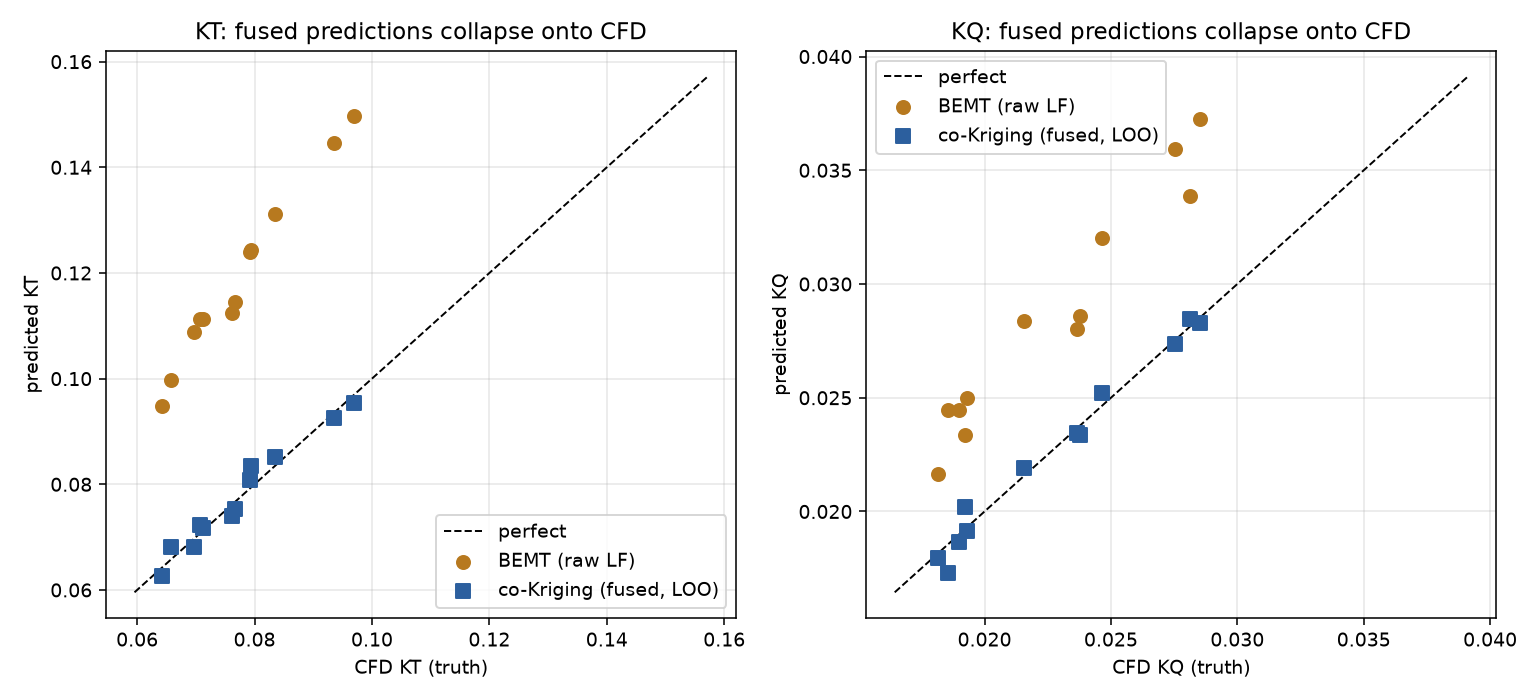
The 2,560 BEMT evaluations from our propeller design search (thinned to ~300 for the fit) were fused with 12 blade-resolved OpenFOAM RANS runs. In leave-one-out, error against CFD fell by 95% for the thrust coefficient and 91% for the torque coefficient compared with raw BEMT.
| Quantity | RMSE BEMT | RMSE fused | Reduction |
|---|---|---|---|
| Thrust coefficient KT | 0.0421 | 0.00193 | −95% |
| Torque coefficient KQ | 0.00612 | 0.00055 | −91% |
What this study does not show
- The design requirement was 380 N of thrust. No CFD run reached it: thrust across the 12 CFD points spans 241.2–257.5 N. BEMT over-predicts thrust, which is exactly what the fusion corrects, and the corrected model shows the shortfall too.
- Re-optimizing on the fused model favoured a different design from the BEMT winner. That design is a surrogate prediction and has not been run in CFD.
- Errors are leave-one-out over 12 CFD points inside the sampled envelope. Outside it, the model drifts back toward BEMT.
04Using it
Where this fits in your workflow
Multi-fidelity modeling is one of the methods in Curlscape Sift. It pays off when you already have, or can cheaply generate, a large set of low-fidelity runs and can afford a handful of high-fidelity ones.
Tell us what your cheap and expensive simulations are. We will check whether they correlate well enough to fuse before anyone builds a model.